Networks from survey data: Creating mock data
Why create a new dataset?
I’d like to do a series of posts looking at social network analysis using primary data (i.e. data collected by yourself.). There are a lot of different examples of when you might want to use a survey to collect data for use in analysing social networks. But that’s for another time.
The purpose of this post is to create a new dataset that can be used in practising social network analysis in future posts. Creating a new dataset in R has a lot of useful advantages. The biggest advantage is that we will have a single dataset that can be used in all future examples when learning SNA with surveys.
Creating a new dataset is also a great learning opportunity because we will reverse engineer a dataset around specific modelling, correlations and otherwise interesting easter-eggs that we can use as learning opportunities in future posts. We will rely on the power of probability statistics to help us get there. And as we make decisions about how to structure our dataset, we’ll learn some important aspects of social network analysis and general data science. We’ll save this for the end though. So, let’s get started!
Building a new dataset
As with most posts on Deltanomics, we’ll use a tidy framework. So, that means loading tidyverse, and we’ll go ahead and load our other SNA workhorse packages.
# For a tidy framework
library(tidyverse)
library(glue)
library(scales)

# Our graphing libraries
library(igraph)
library(tidygraph)
library(ggraph)
An edgelist
The first thing we need to do is create an edgelist structure in our data. Really anything can be used as an edgelist as it’s just two columns that represent an edge is meant to be drawn between adjacent cells. A typical use of surveys in SNA is to look at how information flows between two people and the influence that the information has on sustainable behaviours. So let’s create two columns that would reasonably collect that type of information.
Respondent name
First, we need a column for the respondent’s name or identification. This column length will be the first and primary argument in our function to allow us to create datasets of any size we choose.
For this, let’s use one of my favourite packages randomNames to generate some realistic names.
library(randomNames)

create_sna_data <-
tibble( # let's pull 100 random names to start
    resp_name = randomNames(100,
                  which.names = 'both'))
Information holder
Next, we’ll create a column that holds the name of whom the respondent goes to for information. We want our social network to be complete; meaning that every node in the graph will attribute data. To ensure this happens, we need to take special care that all of the possible nodes are also respondents. In short, the second column of the edgelist needs to be completely contained within the first.
# 1. Make a disconnect graph
g <- make_empty_graph() %>%
  add_vertices(2)

# 2. Run a while loop to ensure that a connected
# graph is created -- this will help smooth over some of the graphing functions for later.
#
while (is.connected(g)== FALSE) {

  g <- create_sna_data %>%
    mutate(info_one = sample(
      sample(resp_name, 80), # create 2nd column
      nrow(.), T)) %>%       # as subset of the
    as_tbl_graph()           # first.
}

# send it back to the original name
create_sna_data <-  g
Now, let’s take a look at how the social network contained within the data looks like.
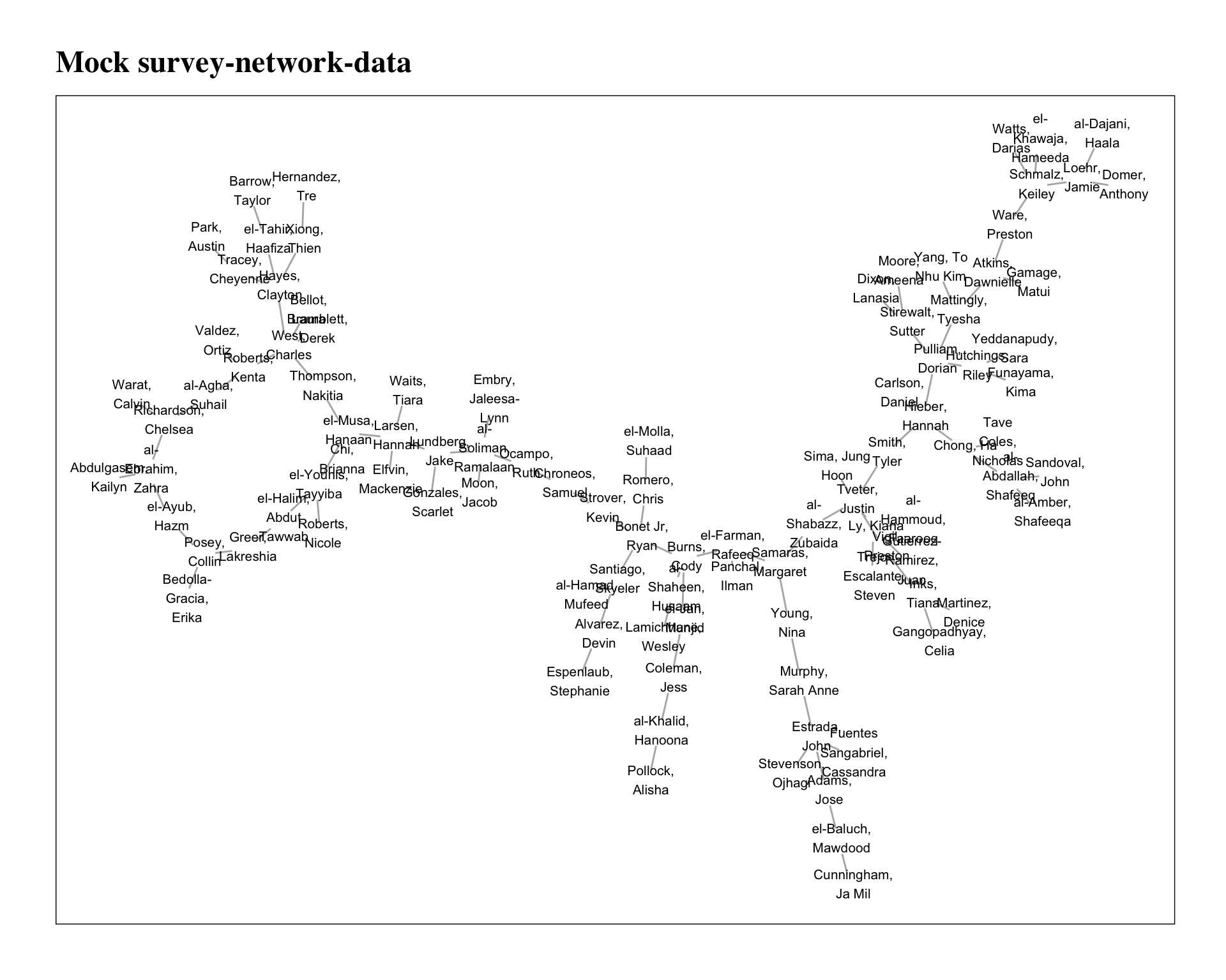 The network should loosely resemble a sparsely connected sociogram, and it should serve our purposes well.
Node & edge attributes
Now that we have our edge list as the first two columns of the data set, we can start to add some node and edge attributes. However, we can’t just randomly create new variables and values because we want a dataset that resembles what we might find in the real world. This means certain variables should be related or correlated with one another. And, because we’re interested in network analysis, a node’s position in the network should also influence their values in key columns. To achieve this, we’ll need to reverse engineer the values based on some graph analysis.
Node attributes
We’ll do some rapid-fire node correlations with some key socio-economic variables.
Income category
create_sna_data <- create_sna_data %>%
  mutate(income_pre_tax = map_chr(degree(create_sna_data), function(x){

    # random normal using degree as the mean
    # and a standard deviation of 2.5
    random_norm <- rnorm(n = 1,
        mean = x,
        sd = sample(2.5, 1, F))

  dollar(abs(random_norm)*15000,
         prefix = '£')
}))
Our dataset has a lot of randomness to it, so it’s impossible to tell what the correlation is. But, it should at least be positive and somewhat linear. There aren’t likely to be many nodes that have the maximum number of degrees, so the variance should drop off as the degree increases (but this isn’t a guarantee!).
A boxplot of showing degree and income is shown below.
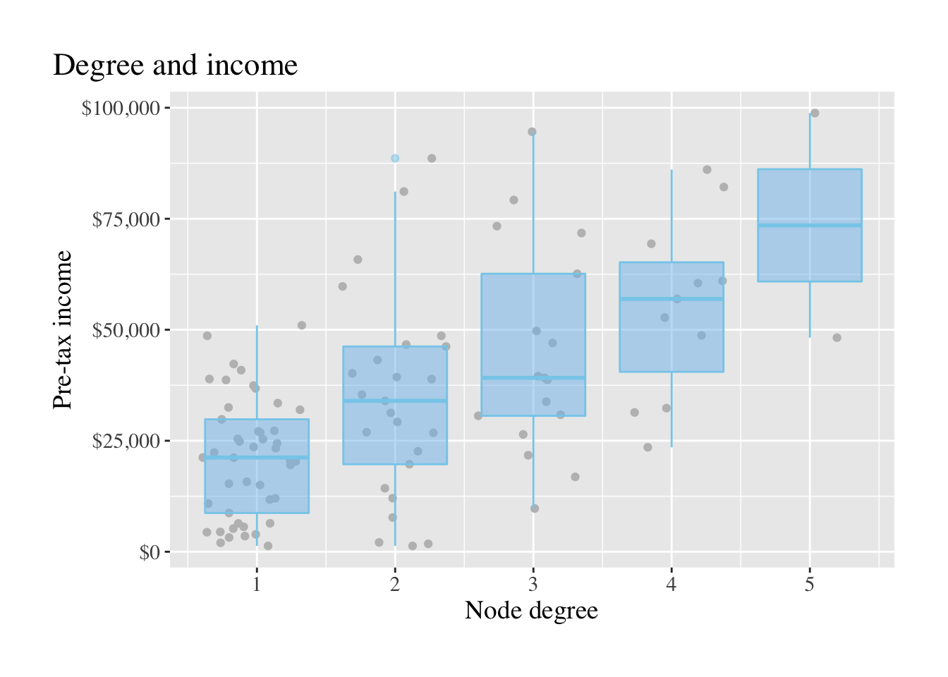 So, the theoretical people in our dataset with more connections to others should make more money, something that, could conceivably be true.
Neighbourhood influence
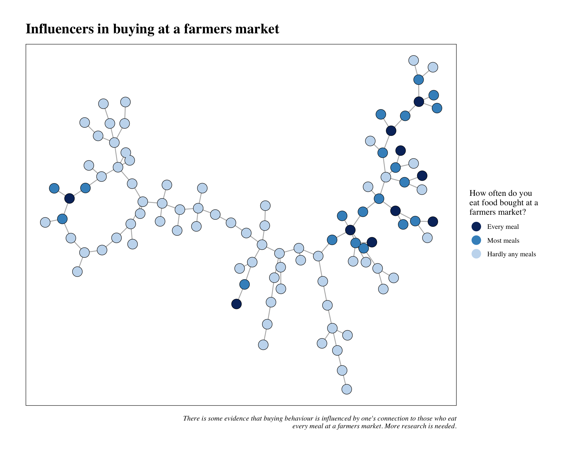
A common question in network analysis is: do nodes behave differently when they are connected to certain nodes. It’s like the old adage ~ if you lie down with dogs you’ll get up with fleas. For this, we’ll pick out some random nodes and have their neighbourhoods adopt a similar value for a question like: do you buy the majority of your fruit and veg from a farmers market?
influencers_df <- map_df(1:10, function(x){

  # pull a random node name
node. <- sample(V(create_sna_data)$name, 1)

  # get the node id, because to_local_neighborhood requires a numeric identifier (this is due to igraph).

 node_id. <- match(node., V(create_sna_data)$name)

 # pull the neighbourhoods of each node from above.
neighbours. <- create_sna_data %>%
  to_local_neighborhood(node = node_id.,
                        order = 1) %>%
    .[[1]] %>%
    as_tibble() %>%
    pull(name)

 # create a tibble of both values for use in the next step

tibble(neighours. = neighbours.,
       centre = rep(node., length(neighbours.)))

})
# create new variable for each value returned above.

create_sna_data <-
  create_sna_data %>%
  mutate(buy_farm_mark = case_when(
    name %in% influencers_df$centre ~ 'Every meal',
    name %in% influencers_df$neighours. ~ 'Most meals',
    T ~ 'Hardly any meals'
  ),
  buy_farm_mark = factor(buy_farm_mark,
                            levels = c('Every meal',
                                       'Most meals',
                                       'Hardly any meals')))
That was a bit verbose and somewhat complicated, but it will be worth it. Let’s take a look below to see how it looks in our new data.
Community influence
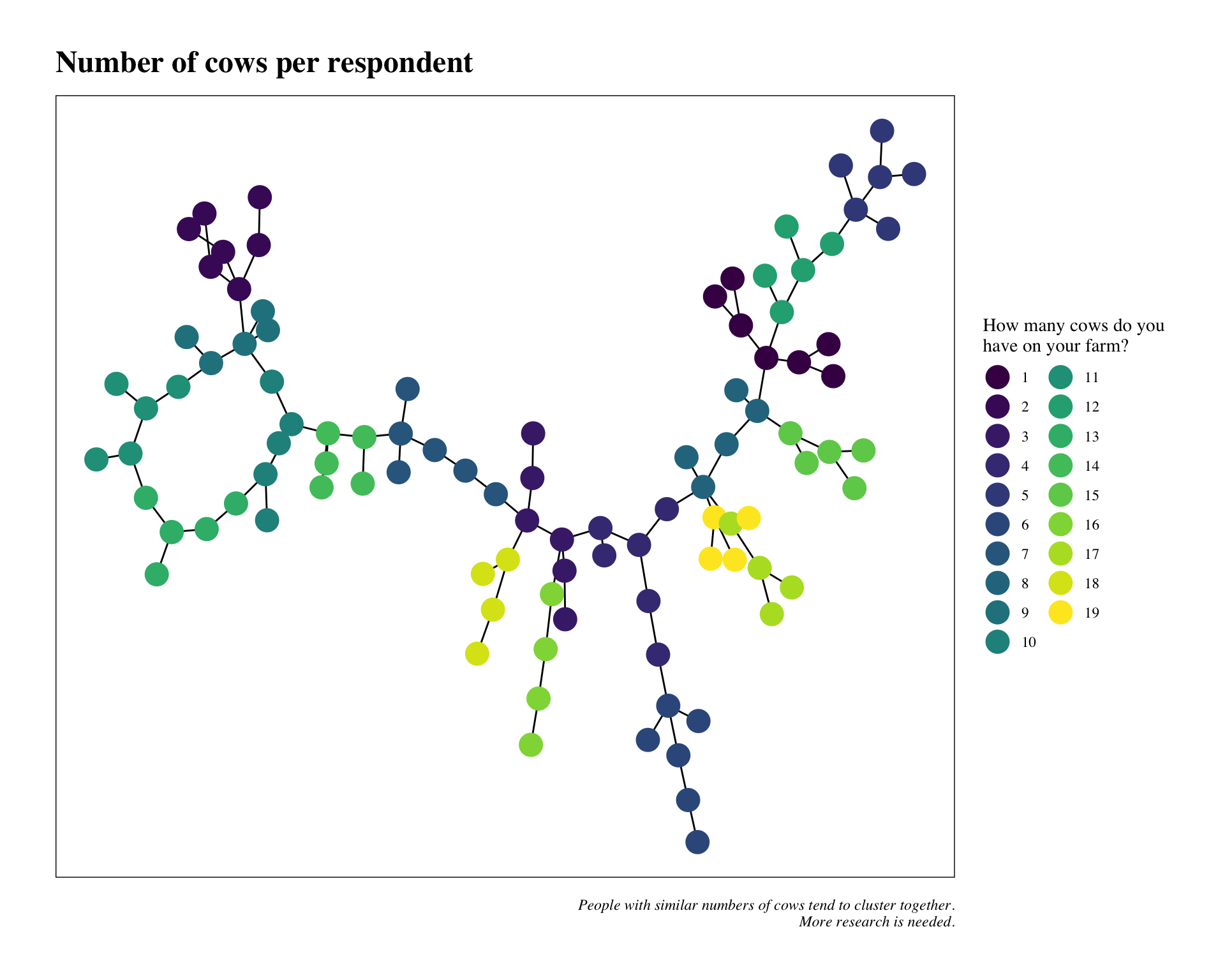
We’ll use a community detection algorithm for the last node attribute for our dataset. This one is a bit easier as we’ll just create a new variable using the group_infomap function from tidygraph/igraph.
create_sna_data <- create_sna_data %>%
  to_undirected() %>%
  mutate(cows_on_farm =
           as.factor(group_infomap()))
The plot below illustrates the communities detected by group_infomap. The only thing we’ve done here is to rename the variable. Easy enough!
We’ll now add edge attributes.
Edge attributes
Edge attributes won’t be as complicated as node attributes for as we’ve aleady identified the relationship between nodes (edges). We’ll just need to think about a variable that would makes sense for trustful communities. One could be that number of cows is related to higher levels of trust (not super likely in the real world, but anything’s possible!). It’s an easy edge attribute to calculate so let’s do that one.
create_sna_data <- create_sna_data %>%
  mutate(trust_score = round(
              rescale(
              as.numeric(cows_on_farm),
              c(1, 10))))
Back to a tibble
We’ve been workig with a tidygraph object for most the post. We’ll want to create a tibble for our purposes. Remember, the goal is to create a mock survey dataset that we can use in the future to learn SNA. So it should look authentic. Let’s do that now.
name_id_df <- create_sna_data %>%
  as_tibble() %>%
  transmute(name,
            value = row_number())

create_sna_data <- create_sna_data %>%
  activate(edges) %>%
  as_tibble() %>%
  gather(key, value) %>%
  left_join(name_id_df) %>%
  split(.$key) %>%
  bind_cols() %>%
  select(resp_name = name,
         recieve_info = name1) %>%
  bind_cols(create_sna_data %>%
              as_tibble() %>%
              select(-name))
All right, that’s it! We can look at our data below; hopefully, it looks like something we might collect in the future for SNA research.
| resp_name | recieve_info | income_pre_tax | buy_farm_mark | cows_on_farm | trust_score |
|---|---|---|---|---|---|
| Roberts, Nicole | el-Younis, Tayyiba | £6,389.69 | Hardly any meals | 10 | 6 |
| Dixon, Lanasia | Stirewalt, Sutter | £23,319.29 | Every meal | 1 | 1 |
| Warat, Calvin | Richardson, Chelsea | £27,098.81 | Most meals | 11 | 6 |
| Chroneos, Samuel | Ocampo, Ruth | £26,924.22 | Hardly any meals | 7 | 4 |
| Lamichhane, Wesley | al-Shaheen, Husaam | £36,799.65 | Hardly any meals | 3 | 2 |
| Loehr, Jamie | Schmalz, Keiley | £73,347.91 | Most meals | 5 | 3 |
Elliot Meador PhD
Research Fellow
My research interests include community resilience, sustainable food systems and computational social science.