Be like me - looping through shortest distance analysis

Last updated on Jun 5, 2020 8 min read R, SNA

Introduction

I’ve been doing some work lately on social networks that exist between organisations or institutions. This is nice as it builds on some of my dissertation work, and I generally find it quite interesting. Networks that form between organisations are often quite powerful, in that they can illustrate where strong areas of like-minded work exist or where new connections might be useful in strengthing one organisation’s influence.

Why like me?

Organisational ties – like personal relationships in business – can be extremely valuable to a firm’s bottom line. These ties are often leveraged and manoeuvred to produce some sought-after result. A few examples might be:

Do I know anyone at Organisation X who might have more information about some big grant schemed about to be launched?

Who in my inner circle has ties to a business who might provide some venture capital for an idea I have?

The notion of leverage’s one’s networks is nothing new. It’s known as social capital theory in sociology and is a well-known tactic taught in business schools. Its applications are too big to get into in this blog post. I’d suggest taking a look at this Forbes article for a bit more information on why this might benefit you. If you’re interested in leveraging one’s ties for their benefit from an academic perspective you can read some of my published articles or read works by James Coleman, Pierre Bourdeau or Robert Putnam from the 1980s and 1990s.

The nitty-gritty

Some data

Now that we know it’s a worthwhile venture to leverage one’ network ties, let’s take a closer look at how we might approach this from a data perspective. We’ll use a portion of the mock data we created in an earlier blog found here. The database created from the code in that blog post is called create_sna_data, and we’ll be using it for the rest of this post.

Finding what we’re looking for

We’re going to be preforming shortest-distance analysis. Shortest distance analysis, also known as shortest paths, is a common algorithm used anytime objects are found within a network. It’s common in logistics work, especially regarding travel along a road or rail network. GIS analysis uses this approach as well. A great example is the Scottish Index of Multiple Deprivation’s use of shortest-distance analysis in looking at access as a form of deprivation in Scotland. Take a look at the SIMD documentation here for an overview.

According to igraph’s documentation:

… [shortest distance] calculates the length of all the shortest paths from or to the vertices in the network. [It] calculates one shortest path (the path itself, and not just its length) from or to the given vertex.

Let’s use the shortest distance function from tidygraph (which implements igraph’s shortest.paths functionality) using a straight forward approach.

Below let’s look at the shortest distance between two nodes.

First, we’ll create a base layout from which to filter for sub-graphs when we want to show a path between two nodes.
Then, we’ll plot the graph using ggraph. ggraph likes the layout matrices to be in tibble form with the column names x and y.

# create a filtering column called id.
create_sna_data <- create_sna_data %>% 
  mutate(id. = row_number())

# use the layout with stress algorythm to create a layout
layout_df <- create_sna_data %>% 
  layout_with_stress() %>% 
  as_tibble() %>% 
  set_names(c('x', 'y') )


## And now the plot
create_sna_data %>% 
  ggraph(layout = layout_df)+ # our layout algorythm from above
  geom_edge_fan(start_cap = circle(2, 'mm'), 
                end_cap = circle(2, 'mm'))+
  geom_node_point(size = 4)+
  geom_node_text(aes(label = id.), 
                 size = 2.25, 
                 color = 'white')+
  labs(title = 'Full network')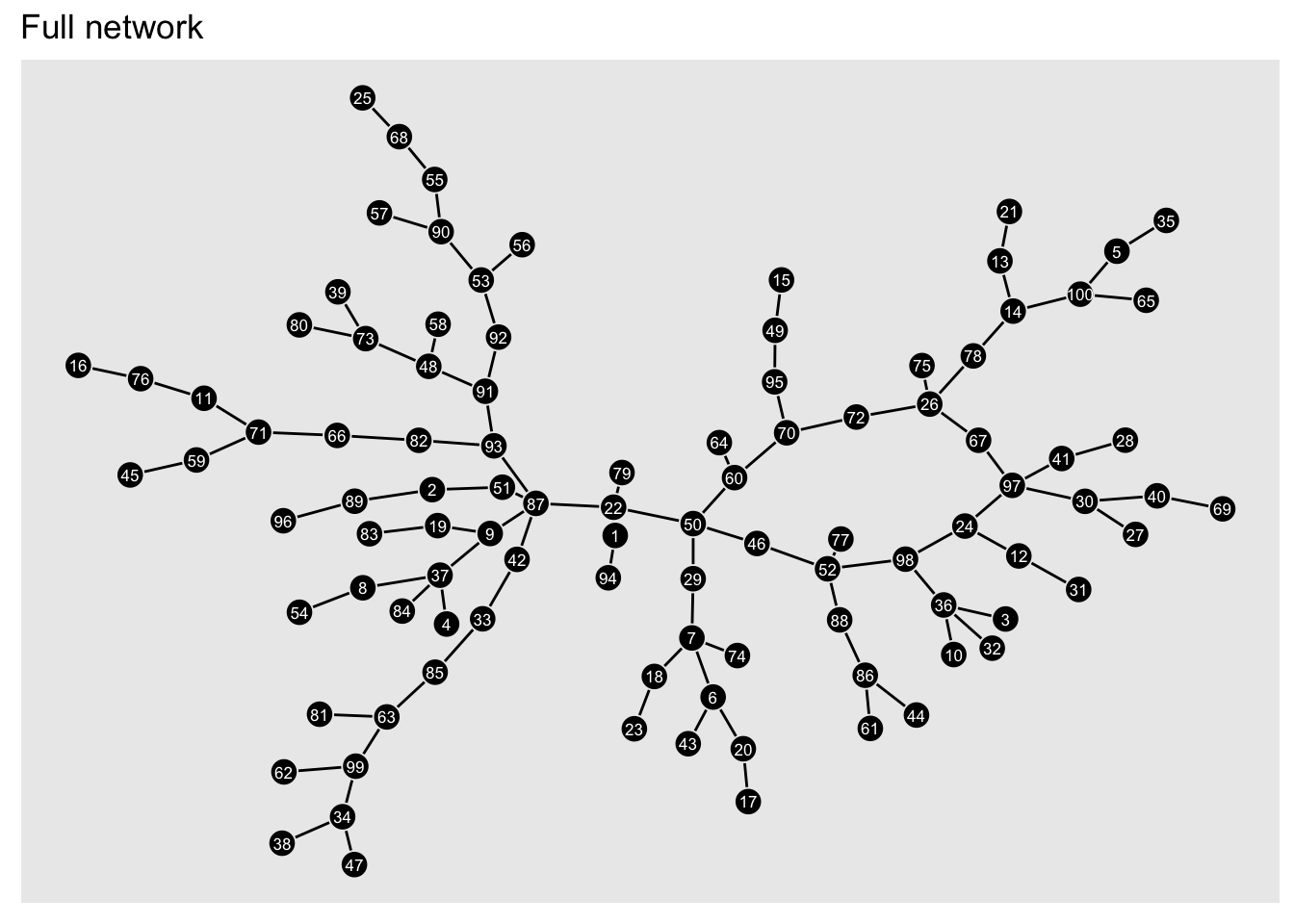

Now, we’ll find the shortest path between two nodes: 75 and 4. We’ll plot the shortest path as a network and lay it on top of the network above so we can visualise the path within the network. To do this, we’ll calculate the layout tibble first and filter it for the shortest paths network using the layout_with_stressfunction from the graphlayouts package. Note that we’ll need to pull our nodes that sit along the shortest path from our layout data frame. We’ll use the slice function in dplyr for this.

create_sna_data_4_75 <- 
  create_sna_data %>%
  morph(to_shortest_path, 75, 4) %>% 
  mutate(selected_node = T) %>% 
    activate(edges) %>% 
    mutate(selected_edge = T) %>% 
  activate(nodes) %>% 
    unmorph()

colors_v <- c('tomato', 
  'skyblue')

names(colors_v) <- 
  c('TRUE', 'Other')


create_sna_data_4_75 %>% 
  mutate(selected_node = ifelse(
    is.na(selected_node), 'Other', selected_node
  )) %>% 
  activate(edges) %>% 
  mutate(selected_edge = ifelse(
    is.na(selected_edge), 'Other', selected_edge
  )) %>% 
  ggraph(layout = layout_df)+
  geom_edge_fan(aes(color = selected_edge),
                start_cap = circle(2, 'mm'), 
                end_cap = circle(2, 'mm'))+
  geom_node_point(aes(color = selected_node),
                  size = 4)+
  geom_node_text(aes(label = id.), 
                 size = 2.5, 
                 color = 'white')+
  scale_color_manual(values = colors_v, 
                     name = 'Nodes', 
                     label = c('Other', 
                               'Shortest path'))+
  scale_edge_color_manual(values = colors_v, 
                     name = 'Edges', 
                     label = c('Other', 
                               'Shortest path'))+
  labs(title = 'Shortest path between nodes 75 and 4')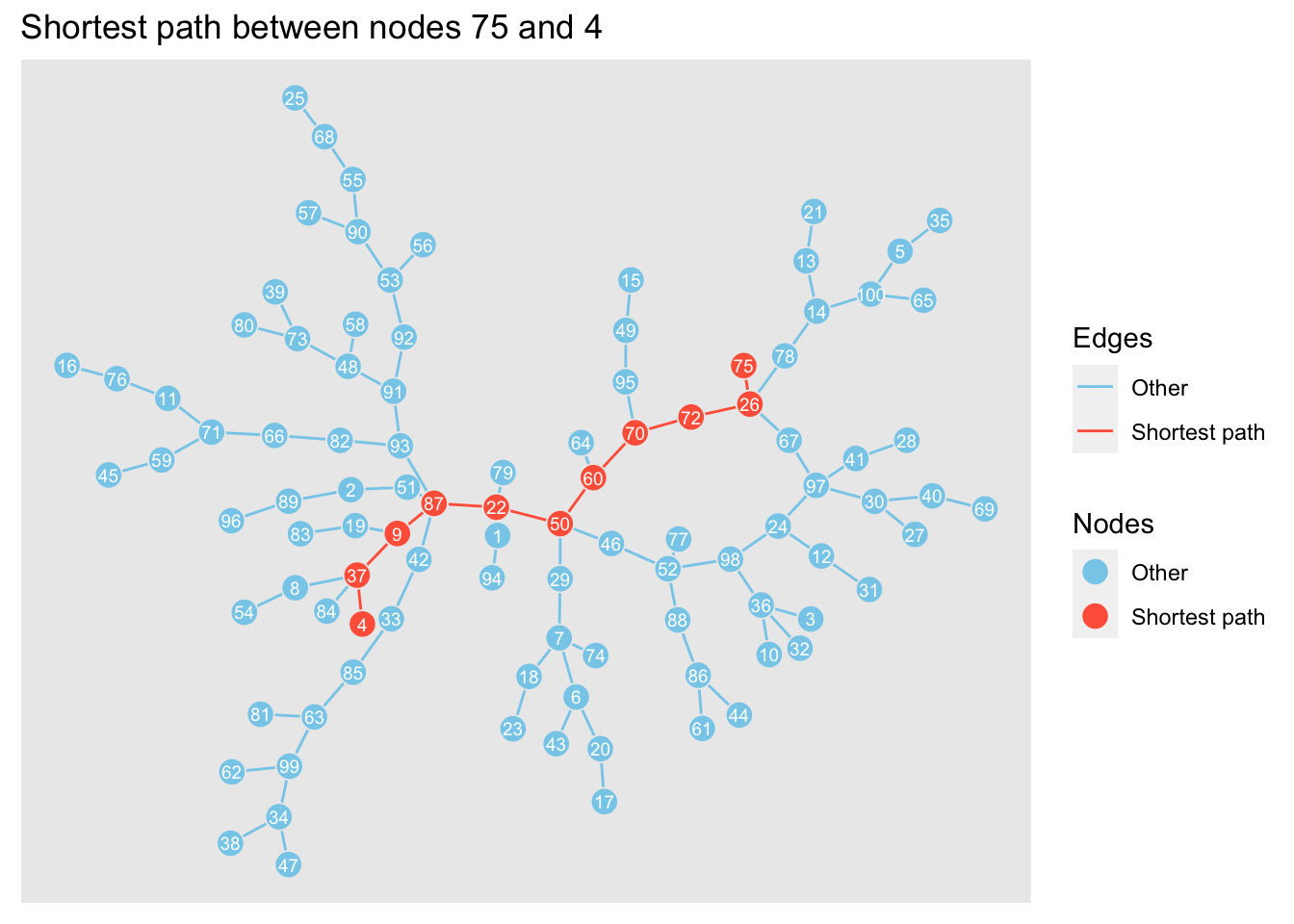

Leveraging networks

The notion of leveraging networks comes from the reality that not every node in a network is available to us to draw resources from. For the most part, a node has a useable relationship with only those nodes in its inner circle – or its one-degree neighbourhood. Now, this isn’t always the case, but as a very general rule with SNA, the further one node is from another, the less influence they have on one another. SNA can help identify which people could put you in touch with some other person based on a set of pre-defined criteria. SNA helps answer the question:

Do I know a dude who knows a dude?

The goal

So let’s suppose our goal is to utilise our social network to find a potential partner to work on a grant with us. The funder of our grant scheme has a real soft spot for loners – i.e. one-degree nodes; maybe because before our funder made it big they used to be a one-degree node themselves. Who knows! Below we see our same network with the one-degree nodes highlighted.

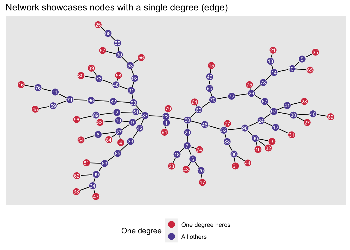
We’ll pretend that we are Le, Brianna (# 87), one of the most well-connected persons in the network (with a betweenness score of 3,088).

We know that we want to partner with a node that has only-degree. We will want to approach as many one-degree nodes as possible, as some will turn us down or might not be available to partner on the grant application.

We also know that we get along with some people better than others and that we’ll have to depend on our relationships to help leverage them. It may sound crazy, but Le, Brianna (ourself) gets along really well with people who buy all their food from farmers markets. So, we’ll use this to our advantage by trying to find as many shortest paths to single-degree nodes that are filled with nodes that buy all their meals at farmers markets. We’ll do this with iterative programming otherwise known as looping. Therefore, our approach is:

Assign a numeric scoring value for the column buy_farm_mark, with more meals receiving a higher score; geodesic distance will also be factored into the score, with nodes further away receiving a higher score.
Identify all shortest paths between Le, Brianna and all one-degree nodes in the network.
Create a scaled score for each path that we can use to decide on who to contact first for partnering on the grant application.

Step 1

# Those who buy every meal from the farmers 
# market get a score of 5, 3 for most meals
# and 0 for hardly any meals.  We'll create 
# a tibble and merge it with data frame. 
farm_buy_n <- 
  tibble(buy_farm_mark = c('Every meal', 
                           'Most meals', 
                           'Hardly any meals'), 
        farm_mark_score = c(5, 3, 0))


create_sna_data_updated <- 
  create_sna_data_updated %>% 
  left_join(farm_buy_n, 
            by = "buy_farm_mark")

Step 2

# get all one-degree node 
one_degree_names <- names(
  which(
    degree(
      create_sna_data_updated) == 1))

# and pull out their names.
one_degree_ids <- 
  which(
    V(create_sna_data_updated)$name %in% 
      one_degree_names)

# Find the max betweeness for the starting node.
max_degree <- which(
  betweenness(
    create_sna_data_updated) == max(
      betweenness(
        create_sna_data_updated)))[1]

## The loop!!
## 
all_shortest_one_degre_paths_ls <- 
  map(one_degree_ids, # our one-degree nodes are here
      function(x){
        
create_sna_data_updated %>% 
          
  morph(to_shortest_path, max_degree, x) %>% 
          mutate(selected_node = TRUE) %>% 
          activate(edges) %>% 
          mutate(selected_edge = TRUE) %>% 
          activate(nodes) %>% 
  unmorph()
})

Step 3

# Create the scores and flatten the list
# into a numeric vector that we can use to 
# subset by.

all_scores <- 
  all_shortest_one_degre_paths_ls %>%
  map(function(x){
    x %>% 
  filter(selected_node) %>% 
  as_tibble() %>% 
  summarise(total_farm = sum(farm_mark_score), 
            n = n(), 
            total_score = total_farm / n) %>% 
  pull(total_score)
  }) %>% 
  flatten_dbl()
  
highest_score <- 
  which(all_scores == max(all_scores))[[1]]

And now let’s take a look at the final results.

Results

Let’s plot our final results using the code below.

color_v_iii <- c('#084081', 
                 '#A8DDB5')
names(color_v_iii) <- c(T, 'Other')

highest_score_g <- all_shortest_one_degre_paths_ls[[
  highest_score]] %>% 
  mutate(selected_node = ifelse(is.na(selected_node), 'Other', selected_node)) %>% 
  activate(edges) %>% 
  mutate(selected_edge = ifelse(is.na(selected_edge), 'Other', selected_edge)) 

highest_score_g %>% 
  activate(nodes) %>% 
    mutate(buy_farm_mark = factor(buy_farm_mark, levels = c('Every meal', 
           'Most meals', 
           'Hardly any meals'))) %>% 
    ggraph(layout = layout_df)+
    geom_edge_fan(aes(color = selected_edge))+
    geom_node_point(aes(color = selected_node, 
                        shape = buy_farm_mark), 
                    size = 3)+
  scale_color_manual(values = color_v_iii, 
                     'Node path', 
                     labels = c('Other', 
                                'Highest score'
                                ))+
  scale_edge_color_manual(values = color_v_iii, 
                          'Edge path', 
                     labels = c('Other', 
                                'Highest score'
                                ))+
  scale_shape('Meals bought from\nfarmers market')+
  labs(title = 'Highest scoring-paths graph')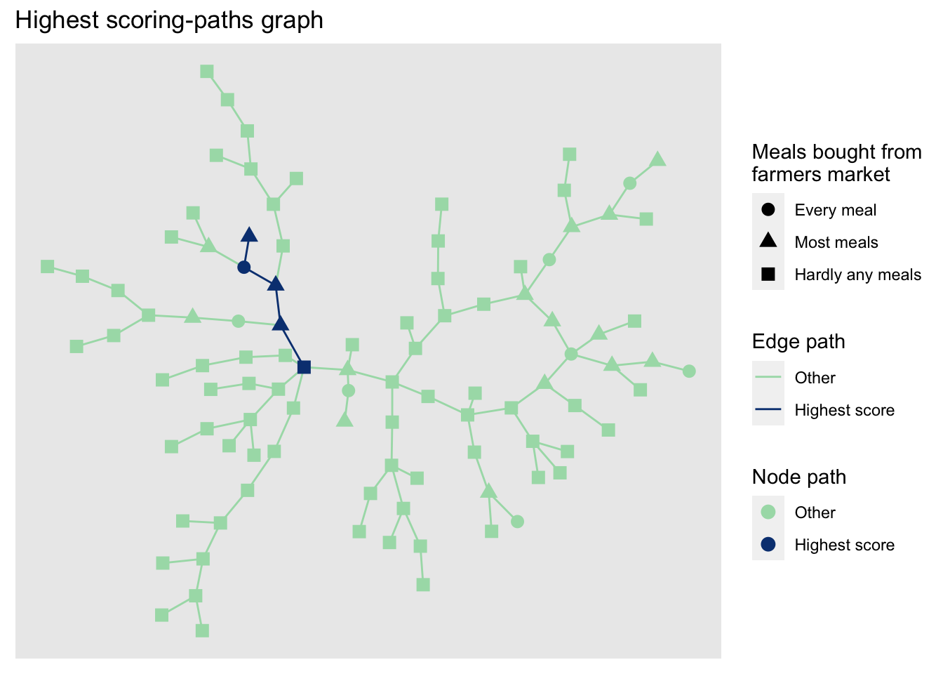

We can see that our approach to identifying the most appropriate project partner favours those nodes that eat every meal with food bought from the farmers market. Of course, this is just a demonstration of how looping can be used with network analysis to find optimum routes within a network.