Covid-19 and Rural Areas in the U.S.
First published on 26-April-2020
Last updated on 16-Aug-2020
Introduction
Now that we are square in the middle of the Covid-19 pandemic, I thought it might be beneficial to look at some statistics associated with the number of cases. We’ll differentiate our analysis by focusing on cases of Covid-19 in rural areas of the U.S. There are a couple of reasons for this: mainly, rural analytics is my speciality, so while I don’t know much about the virus, I do know some about rural societies and economies; we can easily find pertinent data on rural counties; and, we can utilise some cool built-in R functions to help us along the way. Before we go on it’s important to note that:
- I am not a medical doctor or specialist in viral diseases.
- This post is meant to be a learning resource for people interested in looking at the pandemic from a rural perspective.
- Any potential interesting findings must be further investigated before any judgements can be made.
Data
The data for this post comes from two places: Covid-19 cases from the New York Times github; and the USDA Rural-Urban Classification Codes.
Data scientists at The New York Times have been collating data on the number of cases of Covid-19 by county in the U.S.. It is available at their GitHub page, which means that one can easily access and update the data through pull requests. The data can also be downloaded and saved to a local drive.
To get a rural understanding of Covid-19 cases, we’ll use the USDA data on rural-urban classification of U.S. counties, which can be downloaded using the hyperlink above. Many countries have geographical classifications for rural and urban spaces. Usually, a low-level geography is chosen that spans an entire country. A continuum of rural-urban is used to describe each geographical area that goes from very urban to very rural (though not using those specific labels).
So we’ll use those two datasets, join them together and investigate how many cases of Covid-19 are found in rural areas within the U.S..
Analysis
Libraries and themes
Tidyverse packages will be used to do most of the heavy lifting.
We’ll do the data analysis using the dplyr package, and we’ll do our plots with ggplot2.
library(tidyverse)
library(lubridate)
library(janitor)
library(scales)
library(cowplot)

# USDA Rural-Urban classification codes


post_theme <- function(...) {
  theme(
    text =
      element_text(
        color = 'black',
         family = 'serif'),
    axis.text =
      element_text(
        color = 'black'),
    axis.text.x =
      element_text(angle = 45,
                   hjust = 1),
    panel.background =
      element_blank(),
    axis.line.x =
      element_line(
        color = 'black'),
    axis.ticks = element_blank(),
    plot.margin = margin(.75, .75, .75, .75, 'cm'),
    plot.caption =
      element_text(hjust = 0,
                                face = "italic"),
    plot.title =
      element_text(
        face = 'bold'),
    plot.subtitle =
      element_text(face = 'bold'),
    plot.title.position = "plot",
    plot.caption.position =  "plot",
    strip.background =
      element_blank(),
    strip.text =
      element_text(
        face = 'bold')
  ) +
    theme(...) # this bit allows us to make changes using this same function instead of calling two theme functions.
}
# I created a new R-project to house the Covid-19 data in my Documents directory.
covid_county <- read_csv('~/Documents/R/covid-19-data/us-counties.csv')
# Pull in the USDA data from a directory I created in my cloud storage.
rural_urban <-
read_csv('~/OneDrive - SRUC/Data/usda/ruralurbancodes2013.csv') %>%
select(fips,
rucc_2013,
desc = description)Now that we’ve got the data loaded from Covid-19 and USDA Rural-Urban Classifications, we are going to use some of R’s base functionality.
R has two functions that help with general data analysis and joins: state.name, which has all 50 U.S. state names; and, state.region, which has the 50 U.S. state’s categorised into geographical regions.
We’ll use these two functions in a tibble to help join the Covid-19 data with the Rural-Urban Classifications.
state_region <-
  tibble(state = state.name,
         region = state.region)

covid_region <-
  covid_county %>%
  left_join(rural_urban,
            by = 'fips') %>%
  left_join(state_region,
            by = 'state') %>%
  mutate(week =
           floor_date(date,
                      'week'))
Now we have our working data frame called covid_region. It has the following variable names: date, county, state, fips, cases, deaths, rucc_2013, desc, region, week.
We’ll use the description variable to filter out rural counties only.
There are two classifications of rural areas - those that are adjacent to more metro places and those that are not.
Those that are not adjacent to metro areas are adjacent to other rural areas, which makes them somewhat more remote, as people living there need to travel further to get to service centres.
We use the group_by/summarise functionality from dplyr to find the sum of Covid-19 cases and deaths by each week, region and for both rural classifications.
weekly_regions <- covid_region %>%
  filter(str_detect(desc,
                    'rural')) %>%
  group_by(week, region, desc) %>%
  summarise(cases =
              sum(cases, na.rm = T),
            deaths =
              sum(deaths, na.rm = T)) %>%
  ungroup() %>%
  gather(key,
         value,-c(week,
                  region,
                  desc)) %>%
  drop_na()
We’re going to make a fancy-looking plot for this post, something that you might like to share on social media or include in a work report. To help clean up the plot a bit, we’ll use a few approaches that are laid out in the code below.
# each label for the x-axis which we'll use to make some nice looking data labels.
week_n <- weekly_regions %>%
  count(week) %>%
  pull(week)

##------ Wed Jul 29 21:41:05 2020 ------##
# added this to clean up the x-axis
month_n <- week_n %>%
  floor_date('month') %>%
  unique()

# we'll use scale_color_manual with our own color choice
col_v <- c('#3E4A89FF', '#FDE725FF')
names(col_v) <- unique(weekly_regions$desc)

# a simple label_wrap function for the legend
label_wrap <- function(x, n = 25){
  paste0(str_wrap(x, n), '\n')
}

# date labels that use drops today's date into the caption of the plot.
today_date <-
  as_date(Sys.time()) %>%
  format('%d %B, %Y')
OK, now we’ll create the main ggplot that uses facet_wrap to look at each region in the U.S. over time.
weekly_regional_gg <-
  weekly_regions %>%
  filter(key == 'cases') %>%
  ggplot(aes(week,
         value,
         group = desc)) +
  geom_line(size = 1.25,
            aes(color = desc))+
  geom_point(size = 4,
             color = 'grey90')+
  geom_point(size = 3.5,
             aes(color = desc))+
  scale_x_date(breaks = month_n,
               date_labels = '%d-%b')+
  scale_y_continuous(labels = comma) +
  scale_color_manual(
    values = col_v,
    labels = label_wrap,
    name = 'Rural classification')+
  facet_wrap( ~ region) +
  post_theme()+
  labs(caption = 'Severe drop-offs may indicate that data was most recently updated earlier in the week.')
And now we’ll add the labels and annotations.
(weekly_regional_gg <-
  weekly_regional_gg +
  labs(
    title = 'Weekly Total U.S. COVID-19 Cases by Region in Rural Counties',
    subtitle = 'SOURCE: The New York Times, based on reports from state and local health agencies &\nThe USDA Rural-Urban Continuum Codes (2013).',
    x = '\nWeek of',
    y = 'Total',
    color = str_wrap('USDA Rural-Urban Continuum Codes (2013)', 25),
    caption = str_c('By Elliot Meador, PhD; @Elliot_Meador\nNOTE: Last week may not yet be complete.\nProduced ', today_date)))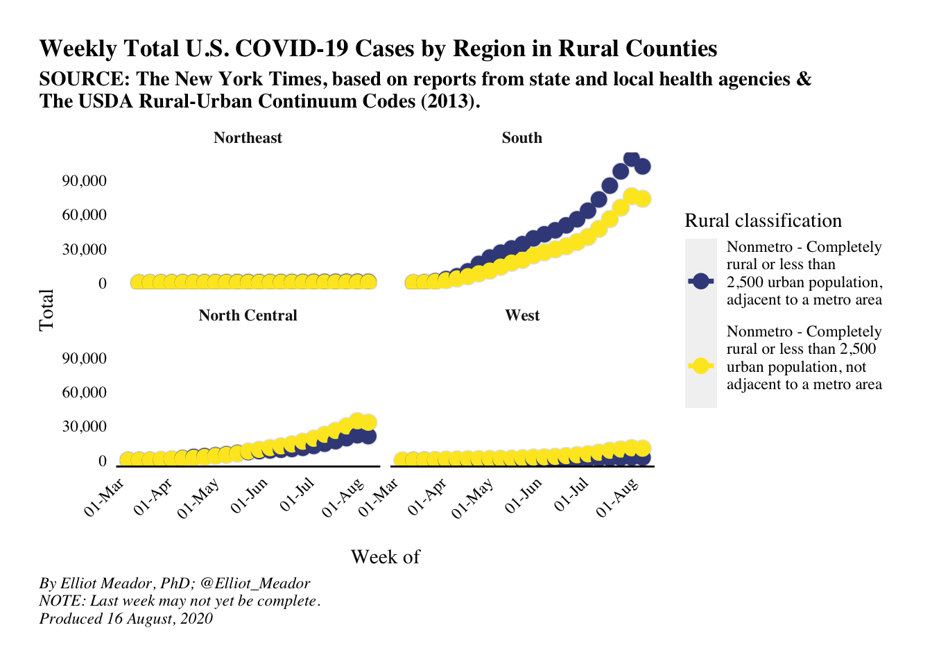
It looks as though rural counties in the south are reporting more cases than the rest of the U.S.. It’s worth investigating the southern counties to see if one state/county is pulling the statistics higher for the entire region, or if the trend is true for the majority of counties. There are a few ways to do this, but the most straightforward is to replicate the plot above but for southern states only. The code below does this.
southern_rural_cases <- covid_region %>%
  filter(str_detect(desc, 'rural'),
         region == 'South') %>%
  group_by(week, state, desc) %>%
  summarise(total = sum(cases, na.rm = T)) %>%
  ungroup()

viridis <- scales::viridis_pal()

southern_state <- southern_rural_cases %>%
  count(state) %>%
  pull(state)

state_cols <- viridis(length(southern_state))

names(state_cols) <- southern_state


labels_df <- southern_rural_cases %>%
  group_by(state, desc) %>%
  filter(week == max(week)) %>%
  ungroup() %>%
  mutate(desc = str_wrap(desc, 35))

weeks_lab <- southern_rural_cases %>%
  count(week) %>%
  pull(week)

southern_plot <- southern_rural_cases %>%
  mutate(desc = str_wrap(desc, 35)) %>%
  ggplot(aes(week, total, group = state))+
  geom_line(aes(color = state),
            show.legend = F)+
  geom_point(color = 'white',
             size = 2.25)+
  geom_point(aes(color = state),
             size = 2,
             show.legend = F)+
  geom_text(data = labels_df,
            aes(label = state,
                x = week,
                y = total,
                color = state),
            size = 2,
            hjust = 0,
            nudge_x = 1.25,
            check_overlap = T,
            show.legend = F)+
  scale_x_date(breaks = weeks_lab,
               date_labels = '%b-%d')+
  scale_color_manual(values = state_cols)+
  scale_y_log10(labels = comma)+
  facet_grid(~desc)+
  coord_cartesian(clip = 'off')+
  post_theme(plot.margin = margin(1.25,
                                  1.25,
                                  1.25,
                                  1.25, 'cm'),
             panel.spacing = unit(2, "lines"))
And just like above, we’ll add our labels seperate.
(southern_plot_ii <- southern_plot+
  labs(title = 'Comparing Covid-19 Cases Across Rural Counties in the Southern U.S.',
       subtitle = 'SOURCE: The New York Times, based on reports from state and local health agencies &\nThe USDA Rural-Urban Continuum Codes (2013).',
       x = 'Week of',
       y = 'Total\nLog10-scale',
       caption = str_c('By Elliot Meador, PhD; @Elliot_Meador\nNOTE: Last week may not yet be complete.\nProduced ', today_date)))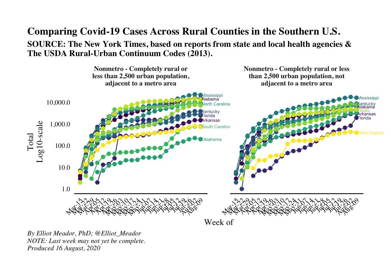
County-level analysis
In the above analysis, we are showing aggregate statistics across states. This gives a good overall understanding of high-level trends, but the next step is to look a bit closer at what happens at a more granular level. Let’s take a look at all rural counties in the U.S. and plot the total cases by the total deaths - which is a common plot I’ve found online.
We’ll only look at rural counties that have at least 10 recorded cases. We’re going to do a twist on a standard scatterplot, where we plot the state abbreviation of the county instead of a simple point. We’ll also colour all abbreviations of the same state in the same colour; this will help draw the readers’ eye to similar states. Lastly, we won’t have a colour legend as this many states will lead to a massive legend that will overpower the plot.
covid_county_rural <- covid_county %>%
  left_join(rural_urban,
            by = 'fips') %>%
  filter(str_detect(desc, 'rural')) %>%
  select(-date, -county, -rucc_2013) %>%
  group_by(fips) %>%
  mutate(tot_deaths = sum(deaths, na.rm = T),
         tot_cases = sum(cases, na.rm = T)) %>%   ungroup() %>%
  filter(tot_cases > 10,
         tot_deaths > 1) %>% # must have at least 10 cases
  select(-cases, -deaths) %>%
  distinct(fips, .keep_all = T)


plot_states <- covid_county_rural %>%
  distinct(state) %>%
  pull()

state_cols <-
  sample(viridis_pal()(length(plot_states)))


names(state_cols) <-  sample(plot_states)


update_date_anno <- paste('Data updated on',
      format(max(covid_county$date), '%d-%b-%Y'))

rural_point_plot <- covid_county_rural %>%
  left_join(tibble(state = state.name,
                   abb = state.abb)) %>%
  ggplot(aes(tot_cases,
             tot_deaths))+
  geom_text(aes(label = abb,
                color = state),
            size = 5,
            show.legend = F)+
  scale_x_log10(labels = comma)+
  scale_y_log10(labels = comma)+
  scale_fill_manual(values = state_cols)+
  scale_color_manual(values = state_cols)+
  post_theme()+
  labs(title = 'Comparing Covid-19 Cases and Deaths Across Rural Counties in the U.S.',
       subtitle = 'SOURCE: The New York Times, based on reports from state and local health agencies &\nThe USDA Rural-Urban Continuum Codes (2013).',
       x = 'Total Cases',
       y = 'Total Deaths',
       caption = paste0('Only counties shown with more than 10 cases and at least 1 death recorded.\nNOTE:Horizontal and vertical axes are on log10 scales.\n',update_date_anno))


rural_point_plot +
  theme(text = element_text(size = 15))+
  annotate('label',
           x = 5000,
           y = 5,
    label = str_wrap('Letters are state abbreviations. Each pair represents a different county within the listed state. State abbreviations are consistently colored.', 40),
    size = 3.5,
    family = 'serif',
    hjust = 0.5)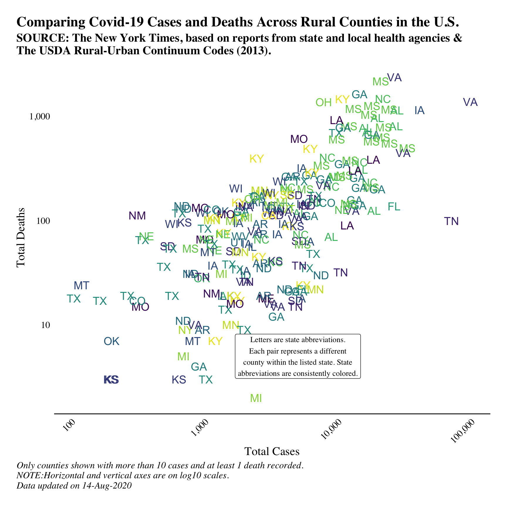
Key Findings
It looks like, at least on the surface of things, that rural places in southern counties report more Covid-19 cases than other rural counties across the U.S.. When we investigated this further by breaking down the states within the southern category, we can see that there is somewhat even spread. That is, one state is not pulling the rest along, which could obscure the actual trend.
I’m from the south-east of the U.S. (Mississippi), and I can say with some certainty that Mississippi, Alabama and Georgia have quite high levels of poverty and ill-health that usually accompanies poverty in the U.S.. It is interesting to see these states reporting higher levels of Covid-19, and it begs the question, “Is there an association between poorer rural places and higher levels of reported cases?” Statistically, I think there probably is (though this needs testing). Even if it is found to be statistically correlated, we still won’t know why we’re seeing these trends until we do more qualitative work in the region to pair with our quantitative findings.
Thanks to the hard work of the folks at the New York Times, we can update our findings over time to see if the trends hold. So stay tuned!
Elliot Meador PhD
Research Fellow
My research interests include community resilience, sustainable food systems and computational social science.